How to Upload Data Frame to R and View It
When I beginning started learning R, it seemed mode more complicated than what I was used to with looking at spreadsheets in Microsoft Excel. When I started working with information frames in R, it didn't seem quite as easy to know what I was looking at.
I've since come to see the light. While there is a fleck of a learning bend to get a handle on it, viewing data in R is infinitely more than flexible than doing so in Excel. In this post, I'll cover the most bones R functions for examining a information set and explicate why they're important.
Understanding how to get a simple overview of the data set has become a huge time saver for me. If you lot aren't familiar with these functions, you lot need to be. If you're anything similar me, yous'll use them showtime for every single data fix you consider.
All of the functions I'chiliad discussing here come in the base R Utils bundle, so in that location's no need to install whatsoever additional packages. Here are the functions, with links to their documentation:
- dim(): shows the dimensions of the data frame by row and column
- str(): shows the construction of the data frame
- summary(): provides summary statistics on the columns of the data frame
- colnames(): shows the name of each cavalcade in the data frame
- head(): shows the first half dozen rows of the data frame
- tail(): shows the last half dozen rows of the data frame
- View(): shows a spreadsheet-similar display of the entire data frame
At present, let's import a data set see how each of these functions works. Offset, hither'southward the code:
### Import a data set on violent crime by land and assign information technology to the data frame "crime" crime <- read.csv("http://vincentarelbundock.github.io/Rdatasets/csv/datasets/USArrests.csv", stringsAsFactors = FALSE) ### Call the functions on crime to examine the information frame dim(criminal offence) str(crime) summary(criminal offence) colnames(crime) ### The head() and tail() functions default to 6 rows, but nosotros can adjust the number of rows using the "n = " argument caput(criminal offense, n = 10) tail(criminal offence, north = v) ### While the outset six functions are printed to the console, the View() function opens a table in another window View(crime) Now, let's take a expect at the output, and then we can see what happens when the lawmaking is run.
First, nosotros'll await at the dim(), str(), summary(), and colnames() functions:

- dim(): In the crime data set, nosotros can see immediately that at that place are only 50 rows and 5 columns. This function is useful, because it tells u.s. whether it would be okay to print the entire data frame to the console. With this information set, it's probably okay. If, however, in that location were five,000 rows and 50 columns, we'd definitely desire to view the data frame in smaller chunks.
- str(): The structure of the criminal offence data set likewise tells us the number of rows (observations) and columns (variables), simply it provides even more data. It tells us the column names, the course of each cavalcade (what kind of data is stored in information technology), and the get-go few observations of each variable.
- summary(): The summary provides descriptive statistics including the min, max, hateful, median, and quartiles of each column. For example, we can run across in the crime data gear up that the boilerplate murder rate across all states is vii.8 for every 100k people.
- colnames(): This office prints a vector of the column names, which can exist useful if you're trying to reference a detail column. For the criminal offense data gear up, we can see that the country cavalcade has no name. Knowing this, we may want to assign it a proper noun earlier going forward in our analysis.
Now, let's accept a look at the head() and tail() functions:
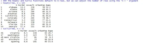
- head(): This function defaults to printing the first 6 rows, only we've decided to phone call the first 10. In the criminal offense data ready, this gives us the data on states Alabama through Georgia.
- tail(): The same equally caput(), except this function prints the cease of the data frame. In this example, we've called the final 5 observations, so we can see the data on Virginia through Wyoming.
Finally, let's accept a look at the window that appears when nosotros call the View() function:
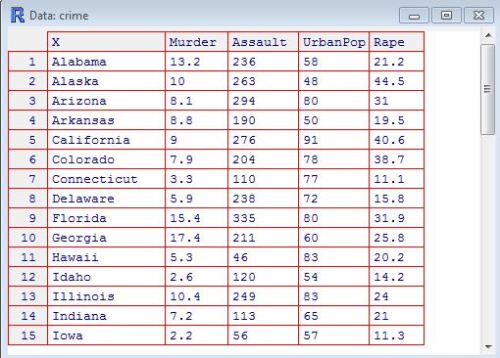
- View(): This window provides vertical and horizontal (if enough columns to justify) whorl bars for you to browse the unabridged data ready. It looks exactly like an Excel spreadsheet–y'all just can't manipulate whatever of the information. (Note: make certain yous use a upper-case letter "V" when calling this role; it's case sensitive).
That's it! Getting comfortable with these functions should arrive easier for yous to work with information frames in a more logical and efficient manner.
Happy viewing!
guerrastratersest.blogspot.com
Source: https://rveryday.wordpress.com/2016/11/29/examine-a-data-frame-in-r-with-7-basic-functions/
0 Response to "How to Upload Data Frame to R and View It"
Postar um comentário